Classical Information Encoding
In the field of computer science, there are numerous methods for encoding information. One such method is the Huffman code, which allows for the reconstruction of the original information after compression and is therefore referred to as lossless compression.
In certain cases, it is possible to disregard a certain amount of data in exchange for achieving a higher degree of compression. Many of you are probably familiar with the JPEG format, which typically sacrifices a portion of the information from the original raster image. The algorithm is designed in such a way that even with some loss of information, the image appears natural, and the human eye usually does not perceive such changes.
By using JPEG, it is possible to reduce the amount of stored information by approximately 10 times while still maintaining a high quality of the image.
Utilizing Neural Networks for Knowledge Storage
Even with the use of modern storage methods, they cannot be considered optimal compared to how the human brain stores information. Our brain cannot boast such high accuracy in reproducing information.
However, it is capable of storing relationships between objects, which allows us to not only recognize objects in an image but also distinguish between what is significant and what is secondary, and relate the obtained information to previous experiences. Instead of efficiently storing raw data, it becomes necessary to store these relationships or functions that can be reused later. Artificial neural networks, or directed graphs, enable us to store data in such a format.
An artificial neural network (referred to as simply a neural network) can be represented as follows:
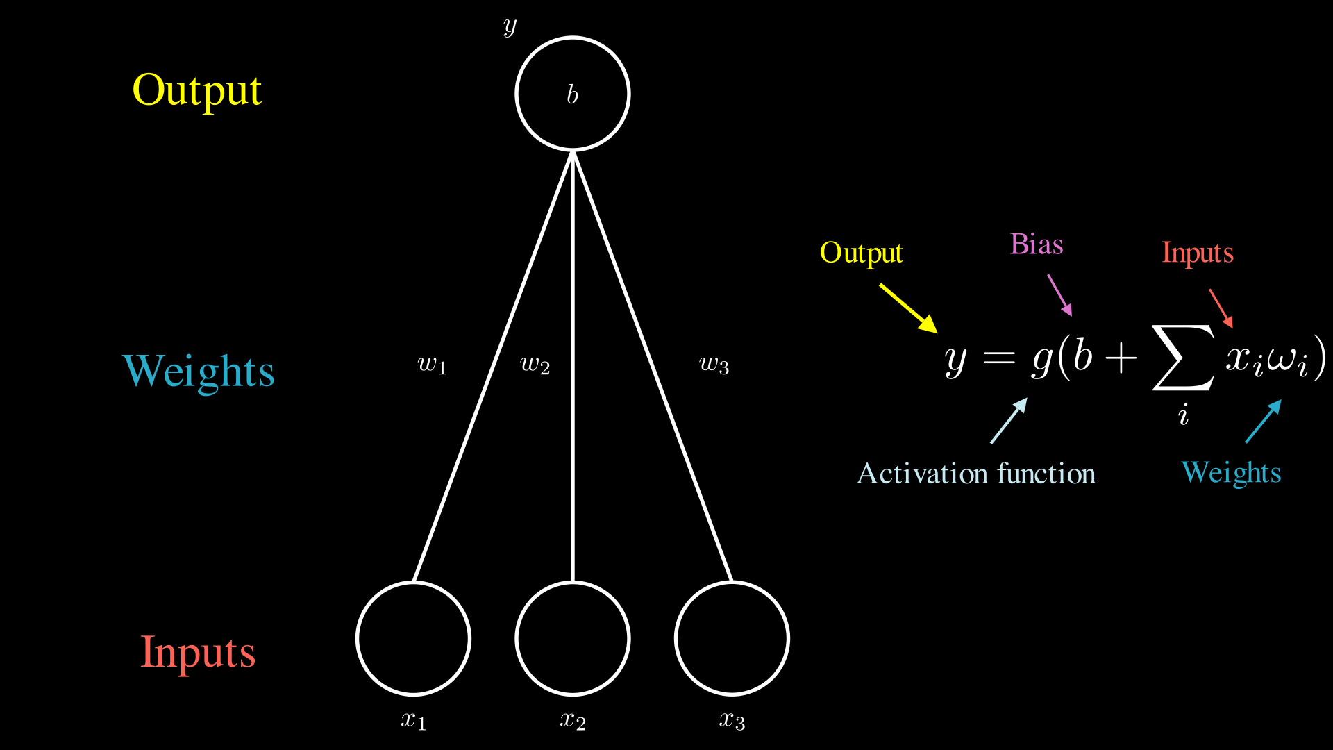 The Structure of a Simple Neuron
where:
- x1, x2, x3 - graph nodes that serve as input data. Typically, they are binary, natural, or integer numbers.
- w1, w2, w3 - graph edges or weights that indicate the significance of the parameters. The larger the value, the more the node influences the final result. Usually, they are rational numbers.
- y - a graph node representing the output data. It is typically a rational number.
- b - bias used for network balancing. The value can be specified either as a node in the network or as a separate input parameter. Usually, it is a rational number.
- g - activation function. It “activates” or “deactivates” the network node and is nonlinear.
The Working Principle of a Neural Network
Let’s start by examining the simplest example depicted above. The calculation of the output can be broken down into the following steps:
- Input nodes receive values, such as 0 or 1.
- All received values are multiplied by their corresponding weights, depicted on the edges.
- The multiplied values are then summed, and the bias value, denoted as ‘b,’ is added to the sum.
- The resulting value is passed through an activation function, which determines the output value.
All the steps described above represent simple mathematical operations, as shown on the right. Of course, in real neural networks, computations are not performed separately for each value. Instead, calculations are done in a vectorized format, which allows for more efficient mathematical operations.
This network demonstrates the working principle of the simplest case and is not typically used in practice. Usually, following the same principle, the network continues, and the node “y,” along with other similar nodes, becomes an input argument for other nodes. In such cases, the node “y” resides within the neural network and is referred to as a “hidden element” or a network parameter. These parameters are what is referred to when specifying the size of a network in terms of parameters since they can encode specific knowledge.
Multi layer Perceptron
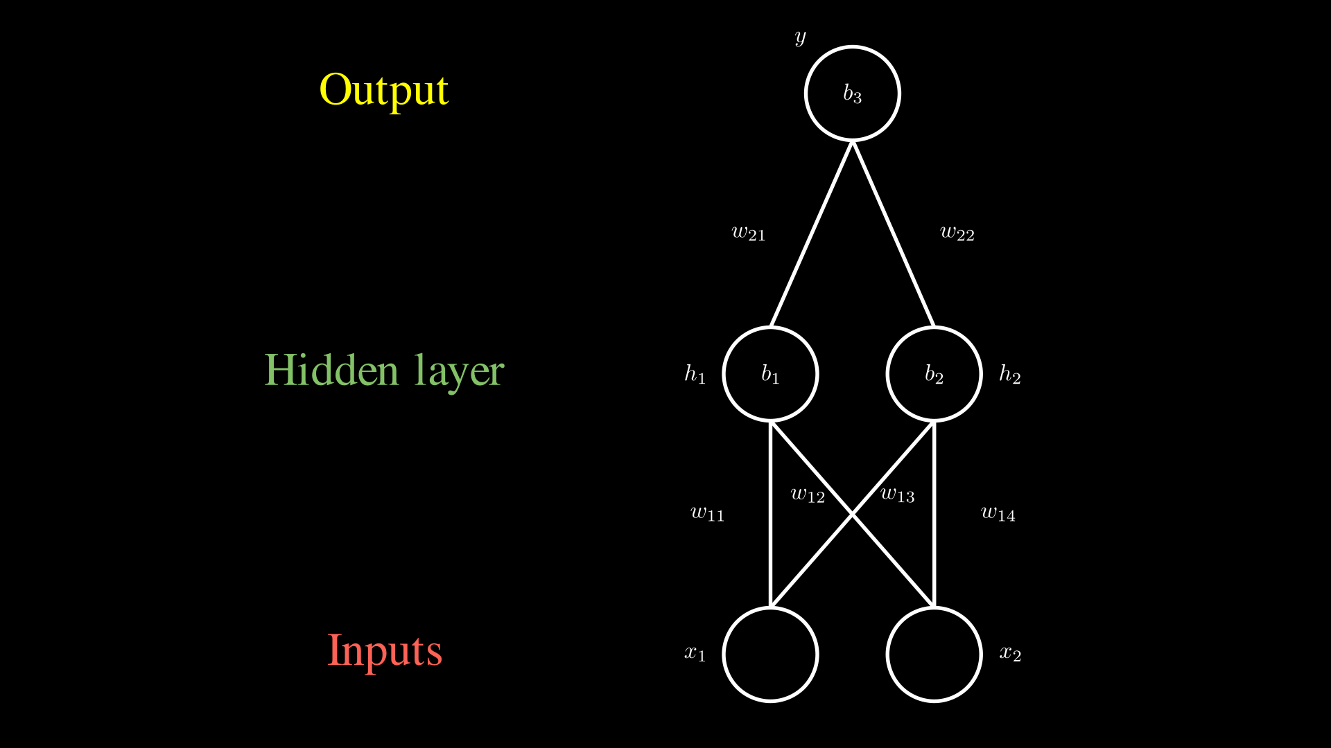
One of the simplest examples of a “working” neural network is the multi-layer perceptron, which is depicted below.
In this network, we can identify three layers: the input layer, the hidden layer, and the output layer. The working algorithm of this network follows the steps described earlier, with the only difference being that the steps are performed for each node in the hidden layer, and then the algorithm is repeated for the output node.
Activation Functions
Before diving into the practical application of neural networks, let’s clarify the concept of activation functions. These functions play a crucial role in activating the neurons of the network, either “turning them on” or “turning them off” in the network’s computations. They also determine the strength of their influence on the final output.
Activation functions can be categorized as linear or nonlinear. Linear activation functions are generally not used in neural networks because George Cybenko proved in 1989 that any feed-forward neural network without internal cycles can be approximated (simplified) to a network with just one hidden layer. This fact imposes limitations on the size and architecture of neural networks, preventing them from becoming truly “deep” by having multiple internal layers.
To overcome this limitation, nonlinear activation functions are employed. These functions allow for larger network sizes and enable the description of more complex data structures. Some of the most commonly used nonlinear activation functions include:
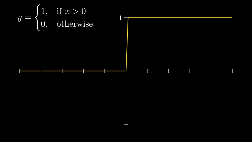
Heaviside Function
The step function is the simplest nonlinear function, with only two possible values: 0 and 1. In the following examples, we will use this function.
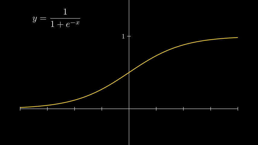
Sigmoid Function
The sigmoid function is one of the earliest activation functions used in neural networks. It gained popularity due to its simplicity and the fact that its output values are bounded within the range [0, 1]. This property allows the direct use of the function’s output as probabilities in probabilistic models, without further normalization or regularization.
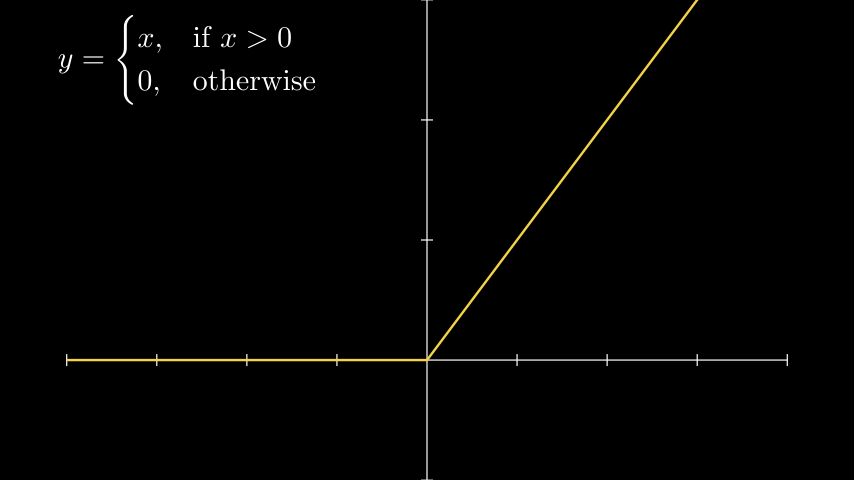
ReLU (Rectified Linear Unit)
ReLU is widely employed in neural networks and remains one of the most popular activation functions to this day. Research has shown that neural networks using ReLU converge faster compared to networks using sigmoid or tanh functions. Furthermore, computing the ReLU function is computationally efficient.
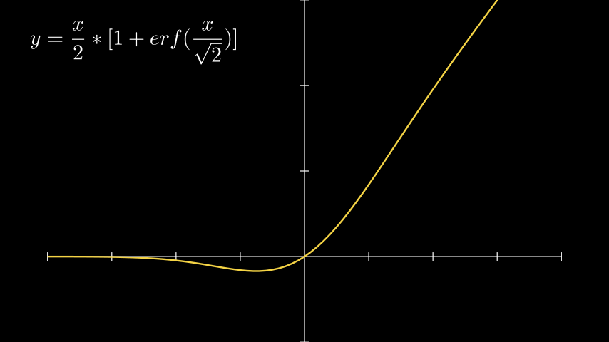
GELU (Gaussian Error Linear Unit)
No, this activation function has nothing to do with the hero Gelu from the “Heroes of Might and Magic” game series. The GELU activation function, as described in the research paper, is similar to ReLU but with a smoother transition from negative to positive values. While GELU asymptotically approaches ReLU for positive values, it is not a linear function like ReLU. This characteristic contributes to faster convergence of neural networks during training.
Activation Functions in Practice
Let’s consider an example where we have a set of data points that can be plotted on a coordinate plane. 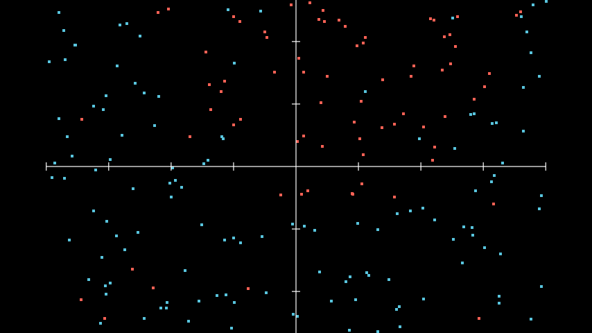 Example data for classification
Our neural network needs to learn how to classify the data points in this set. At first glance, it seems that a linear model wouldn’t be able to accurately separate the data into two classes. Let’s try using a linear activation function for this dataset.
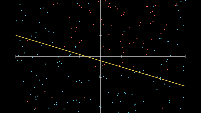 Using a linear function to solve nonlinear problems
As we can see, the linear activation function was able to correctly separate and classify most of the points. However, a significant portion of instances were misclassified due to the simplicity of our function.
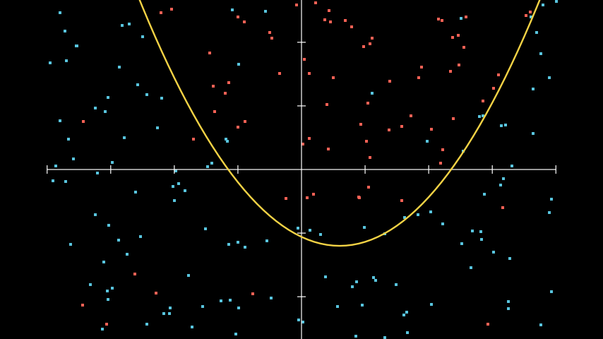 Applying a nonlinear function to solve nonlinear problems
By incorporating nonlinearity, we can draw a more precise boundary between the two classes. This also allows us to build models with a larger number of parameters, enabling us to describe more complex data.
XOR
Let’s explore the application of a simple neural network that can perform the XOR (exclusive OR) function. The possible input values and their corresponding results can be represented in the following table:
| x1 | x2 | y |
|---|---|---|
| 1 | 1 | 0 |
| 1 | 0 | 1 |
| 0 | 1 | 1 |
| 0 | 0 | 0 |
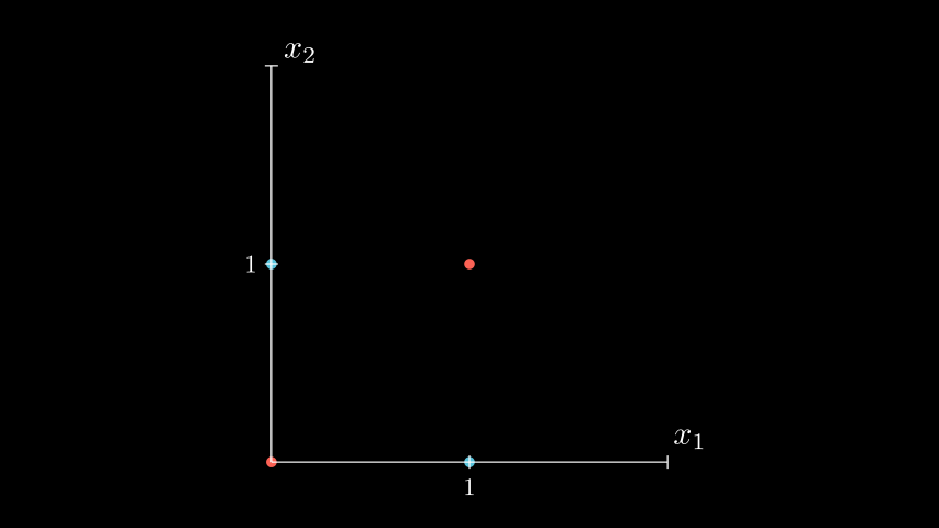
As we know, the XOR function is not linearly separable. This means that it is impossible to draw a single straight line that can separate all the points in a way that red points are on one side and blue points are on the other.
(Of course, you don’t have to take my word for it. Those interested can try to prove or disprove this as a homework assignment.)
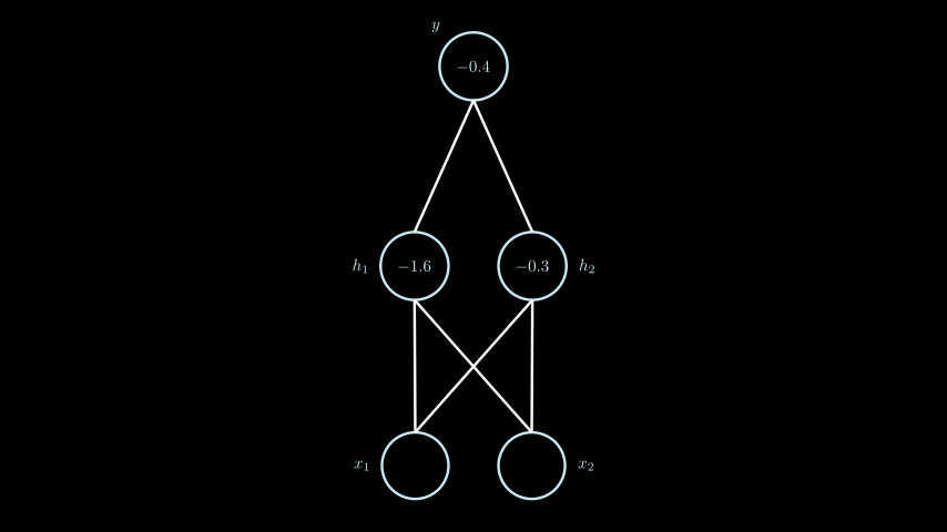
To solve this problem, we will use a multi-layer perceptron with the same structure as shown above. This time, we will use real values.
We will use a simple Step function as the activation function. The function’s output is displayed as either green when the value is “1” or red when the value is “0”.
For simplicity, in this example, all computations are performed sequentially for each layer of the network and each individual node. Once a layer’s calculations are complete, the result is passed to the next layer until it reaches the output layer y. Typically, for faster computation, these calculations are performed in a vectorized form.
Conclusion
In this article, we have described the algorithm of a simple multi-layer perceptron and demonstrated its usage as an XOR function.
In the upcoming articles, we will explore the gradient descent algorithm, which allows us to train a neural network. We will also discuss optimization methods and implement the training algorithm in practice. Stay tuned for more exciting insights and practical implementations!
